Megiddo 2D LP Visualizer was a peronal project for CS6703 Computational Geometry
Try playing with the visualization here.
Project Summary
Implemention of Megiddo’s 2D Linear Programming algorithm that computes the optimal point in linear time.
⚠️ This specific implementation’s main purpose is to visualize the step by step process and runs slower than O(n). See details in Resources section.
Visualization by color coding using Javascript Canvas.
About The Project
This is the course project for CS-6703 Computational Geometry under guidance of Prof. Boris Aronov at NYU Tandon School of Engineering.
The Algorithm
Megiddo’s algorithm is a deterministic linear programming algorithm that runs in O(n) time designed by Dr Nimrod Megiddo. I am implementing its 2D straight line version for my project. Without the loss of generality, rotate the constraints so the target vector is pointing vertically downwards. Then the aim is to find the point which has the lowest y value in the feasible region. The algorithm does the following things:
- Pair the lower constraints arbitrarily and calculate intersection point for each pair
- Find the median x value of the paired intersections
- Deploy a vertical test line at the median x value, get top lower constraint(s) and bottom upper constraint(s). In the following content of the report I will used their abbreviations–TLC and BUC.
- Discard one constraint every pair for half of the intersecting pairs, depending on the information returned by the test line.
- Do 1-4 again, but with constraints on the other side. Or go to 6 when both sides have only constant amount of constraints left.
- Bruteforce the result.
Implementation Details
Technically speaking the whole project should have been divided into a implementation part and a visualization part, but I did them together to make the process easier for me.
I split the steps to these smaller functions:
median():get the median from an array of numbers (copied from online, the code uses sorting instead of rank selection, as the main purpose of this project is visualization, let’s pretend it can select median in O(n)).draw(),onmousedown(),onmouseup(),onmousemove()are the functions that allow drawing on the board.process_line(): takes the coordinates of two points and returns (a,b) after calculating the line in y=ax+b form by solving the equations ax1+b=y1 and ax2+b=y2, which result in a=(y2-y1)/(x2-x1), b=y1-a*x1get_full_line(): calculates the segment to be displayed on the board (extends to the boundary of the board).(extend the originally drawn segment so that x0=0 and x1=1500 to look like a straight line on the board).calculate_intersection()that calculates the intersection point of two lines by solving a1x+b=a2x+b.test_line()1) deploys the test line that returns the TLC(s) and BUC(s); 2) draws the test line and Highlight TLC and BUC with different colors on the board. For the lower constraints:pair(): pairs the remaining lower constraints arbitrarily.update(): clears the board and then draws the current subproblem (all the remaining constraints).update_pair(): draws intersection of the current pairs on the board.update_discard(): draws 1) the intersection points of the pairs that will have one of the constraints discarded 2) the constraints that are discarded in the current iterationget_median_intersection(): finds the median x value of the pairs’ intersections.discard_left()anddiscard_right(): discard half of the lower constraints on one side based: if discard on left, discard the one in a pair with smaller derivative for it will be forever below the other on the right of the intersection; if discard on right, discard the one in a pair with larger derivative for the same reason.discard_constraints():takes the result of test_line() and uses the TLC and BUC to determine which discard function to call.For upper constraints, there is a similar set of functions that includes
_upperin their function names. However, there are some differences indiscard_left_upper()anddiscard_right_upper()comparing todiscard_left()anddiscard_right(): when discarding upper left, discard the one with larger derivative because the one that will be lower to the right of the intersection is more constraining, vise versa fordiscard_right_upper().brute_force()calculates the optimal point when both sides have <= 5 constraints remaining. As the optimal can only be at the intersections of two lower constraints or a lower constraint and an upper constraint, check if each of the intersections are feasible and return the one with the smallest y value.step_lower()callsdiscard_lower()and handles the displays if there are more than 5 lower constraints remaining.step_upper()does the same thing, but with upper constraints.step()is the function that triggers when the run button in index.html is pressed, it determines which side to process, displays result if optimal point if found or does not exist and displays console messages.
Unexpected Difficulties and Complications
- When dealing with both sides of the constraints, it is not sufficient to deal with one side after dealing with another. Because
test_line()costs O(#remaining constraints) and not alternating would makestep()cost quadratic time. - At first, I wanted to display every paired intersections on the board. However, as the intersection coordinates can be far away outside the board, I decide not to display them. This visualization is only focusing on the intersections inside this board and only the inputs that make the intersections inside the board will display a better visual presentation of the algorithm.
- There are some edge cases with
test_line(), namingly when there are multiple TLCs or multiple BUCs.- If in feasible region, multiple BUCs does not affect the decision
- If multiple TLCs, an early detection of the optimal point may happen when there is at least one TLC with positive derivative and another with negative derivative at test line, because local minimum is global minimum in straight line linear programming problem.
- If not in feasible region
- if there are multiple TLCs
- The side where feasible region may exist can be determined by comparing min(TLC’) to max(BUC’) (highest TLC and lowest BUC on the left) and max(TLC’) to min(BUC’) (highest TLC and lowest BUC on the right). If min(TLC’) > max(BUC’), it means at some x value to the left, the lower constraint with a=min(TLC’) will be below the upper constraint with a=min(BUC’), thus there might be a feasible region on the left, so it is safe to discard on right. Vise versa with max(TLC’) < min(BUC’).

- In this case no feasible region exists be cause neither min(TLC’) > max(BUC’) or max(TLC’) < min(BUC’) is true. This means the top lower constraints are constraining the feasible region in a convex region strickly above bottom lower constraints so no feasible region exists.
- If ther are multiple BUCs:
- As we are already using max(BUC’) and min(BUC’) in the case of dealing with multiple TLCs, they are already taken care of.
- if there are multiple TLCs
- If in feasible region, multiple BUCs does not affect the decision
- The console messages are also causing some confusions. I respect UIUX people more and more everyday.
Built With
Resources
- Codes/Tools from online
median(): function that calls JavaScript’s built in sorting function. ⚠️ In an O(n) implementation a function that finds the median of an array in O(n) is needed. Examples include Deterministic Rank Selectiondraw(),onmousedown(),onmouseup(),onmousemove()andcanvascomponent ofindex.html: the functions and web component that enables the drawing effects is from https://stackoverflow.com/questions/49885020/drawing-a-straight-line-using-mouse-events-on-canvas-in-javascript. As you can see by following the link, it is a very basic drawing board. It does not even provide functions to store the lines as coefficients.- This README template,
Best-README-Template, from https://github.com/othneildrew/Best-README-Template. - Deployment of the webapp is powered by CloudFlare.
- Understanding the algorithm
- homework materials by Prof. Boris Aronov at NYU Tandon School of Engineering.
- course notes by Prof. Greg Aloupis at NYU Tandon School of Engineering.
Getting Started
To get a local copy up and running follow these simple example steps.
Installation
Clone the repo
git clone https://github.com/HengningZhang/Megiddo2DLP_visualization.git
Open index.html in your favorite brower and it will be ready to go.
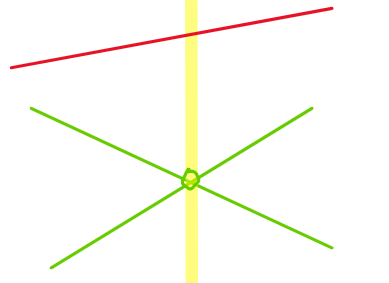
To use it as a webapp, go to Megiddo 2D LP Visualizer. Draw the upper constraints first, they will appear in red lines. Click the save button to save them. Then draw the lower constraints, which will appear as green lines. Then just click run to display the running process of the algorithm step by step. The color coding notations are shown in the legend on the left. The console on the top left will show what is being done in each step. When it shows “Optimal found” or “no feasible region”, it ends.
License
Distributed under the MIT License. See LICENSE in GitHub for more information. Open source hell yeah!